NISAR’s Calibrated Data Is Public: Building a Production SAR Workflow Across NASA and ISRO

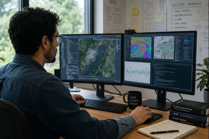
It’s late August 2026 and your project to build an operational SAR processing pipeline has run into a familiar snag: NASA just announced that NISAR’s calibrated L-band data (post-June 17 acquisitions) are now public, and ISRO’s S-band SAR products (starting July 8, 2026) are live on Bhoonidhi. This means data access methods have changed overnight. A naive download of SLC files from the wrong portal, or ignoring polarization and orbit metadata, can break months of work. In practice, a data engineer in this situation would need to review interfaces, update credentials, and re-architect the workflow to unify NASA’s Earthdata/ASF pipeline with ISRO’s Bhoonidhi.

This guide is written for a remote-sensing scientist or engineer (the sort described in Remote Sensing Scientist/Engineer: Earth Observation in the AI Era) who must deliver a robust NISAR SAR analysis now. We’ll show how to discover and download NISAR L- and S-band products (through NASA Earthdata/ASF and ISRO’s Bhoonidhi), how to pick the right product levels, preserve radiometric/polarimetric calibration and geometry, process interferograms and time series, scale up in the cloud, and validate everything. The goal is a reproducible pipeline and a portfolio-ready project (for example, mapping ground deformation or soil moisture with NISAR data). By the end, you’ll have a detailed roadmap of first steps, decisions, and checks (for instance, verifying orbit alignment or polarization order) to avoid common failures and deliver reliable SAR outputs. Along the way, we’ll cite mission specifications and access details. NASA/JPL’s NISAR mission documentation describes a roughly 240 km swath and 12-day revisit, and we’ll point to tools (ASF Search, Earthdata APIs, AWS S3) and training resources. The hardest part will be avoiding the temptation to treat the new mission as just a single-band “fancy Sentinel” dataset; instead, think in terms of a production workflow across two ecosystems, with formal versioning and test criteria.

1. Why Public Calibrated NISAR Data Changes the Workflow

NISAR’s arrival is a paradigm shift. For the first time, a dual-frequency, fully-polarimetric SAR mission is delivering open, radiometrically and geometrically calibrated data. This contrasts with most missions where users had to calibrate or fuse multiple sensors. Key changes:

• Dual L- and S-band: One mission, two frequencies, four polarizations per frequency. L-band (24 cm) penetrates vegetation and soil, ideal for subsidence and biomass; S-band (9.4 cm) is stronger in rain/cloud and provides complementary polarimetry. This adds flexibility but also complexity: our pipeline must handle data from two instruments with possibly different calibration baselines. NASA and ISRO note that NISAR’s 12 m reflectors and SweepSAR beamforming give a ~240 km swath at 7–15 m resolution (depending on direction), revisiting Earth every 12 days. In practical terms, this means an enormous data volume (~10^4 km² per scene) from each pass, and a dense temporal stack (2 passes per 12-day cycle, ascending + descending). The workflow must scale accordingly.

• Fully calibrated (PROVISIONAL) products: Unlike pre-launch or prototype releases, the just-published NISAR data are calibrated for science. NASA’s announcement (July 21, 2026) confirms that ASF/DAAC is releasing calibrated L-band science data (June 17 onward). ISRO’s release page also emphasizes calibrated S-band products (current baseline v1.4) from July 8, 2026. In practical terms, that saves us from needing to apply raw calibration constants, but it also means we must pay attention to calibration updates. Both agencies warn that residual issues (e.g. radiometric banding, RFI in low-SNR areas) may remain, so validation steps are still essential. Note the timeline: NASA/ASF provided ~100,000 pre-calibration L-band products in Feb 2026 for testing, but the full global archive of calibrated L-band was scheduled for July 2026. Therefore any pipeline built now should plan to re-run once final calibration and reprocessing (planned fall 2026) are complete.

• New access ecosystems: Data now arrive through two channels. NASA’s L-band is on the ASF (Alaska Satellite Facility) DAAC and Earthdata, discoverable via NASA’s Earthdata Search, Vertex, and ASF APIs. ISRO’s S-band goes through Bhoonidhi (the NRSC data portal), with its own search-and-order interface and an API (for authorized users). Each has different credential requirements (NASA Earthdata login vs. Bhoonidhi account), and different formats (global L-band vs India-centric S-band mosaic). We’ll address both below, but the takeaway is: you can’t treat NISAR data like just another Landsat or Sentinel feed. You must integrate two pipelines carefully.

• High volume and cloud availability: Processing must embrace cloud scale. NASA confirms NISAR data sit in an AWS S3 bucket, meaning we can process in AWS/GCP without downloading everything (saving time and bandwidth). But it also means jobs must be automated and containerized to handle big data. Our workflow will use cloud APIs and services for efficiency, but still provide full traceability (we’ll keep versioned logs, checksums, and metadata for every step).

In short, public calibrated NISAR changes our workflow by adding data, new tools, and a demand for formal data engineering. We will pivot from a single-sensor approach to a multi-ecosystem production pipeline, automating NASA Earthdata and Bhoonidhi downloads, keeping track of calibrations/polarizations, and building fully reproducible processing steps.

2. Understand the L-Band and S-Band Product Ecosystems

Before coding, get oriented to the product landscape. Both NASA and ISRO define multiple product types (L1, L2, interferometric, etc.), but the naming and availability differ between L- and S-band.

NASA Earthdata and ISRO Bhoonidhi Access Paths

NISAR data can be accessed through several complementary tools. On the NASA side, Earthdata Search (web), ASF’s Vertex SAR discovery tool, the ASF Search REST API, and the Python asf_search package all allow users to find L-band products. For example, ASF’s documentation notes: “NISAR products can be discovered through NASA’s Earthdata Search or ASF Vertex. Programmatic access is also available through ASF SearchAPI and the asf_search Python package”. These tools support interactive searches and scripted queries (see Section 4 for details). Once you have Earthdata login credentials, you can use asf_search to query by date, orbit, processingLevel (e.g. RSLC, GCOV) and more. For advanced cloud workflows, you may also access the ASF S3 archive directly (AWS “SearchAPI” and open bucket access) to stream data instead of downloading.

In contrast, ISRO’s S-band products are fetched via the Bhoonidhi portal. After registering for a free account, users can use the Browse & Order interface to search by footprint, time range, product type (Level-1 RSLC, Level-2 GSLC/GCOV, interferogram, offset, etc.), and place orders for download. For automation, ISRO provides a Bhoonidhi API for authorized users (request access through the portal’s support channel). Note that Bhoonidhi also offers built-in utilities: an HDF5-to-GeoTIFF (COG) converter and a QGIS-based SARPOL tool for polarimetric decomposition, which can simplify geocoding NISAR HDF5 outputs on the fly.

To summarize, here are the main access paths:

        NASA/ASF (L-band):

•        Web Search: Earthdata Search portal (requires NASA EDL login).

•         Vertex: ASF’s SAR-specific search interface.

•         APIs: ASF SearchAPI REST or asf_search Python.

•         Cloud: AWS S3 (public bucket).

Credential: NASA Earthdata (EDL) account (see Section 4).

ISRO/Bhoonidhi (S-band):

•         Web Order: Bhoonidhi Browse & Order (registration required).

•         APIs: Bhoonidhi REST API (requires separate request; contact NRSC).

•         Tools: HDF2TIFF (for COG), SARPOL QGIS for analysis.

•         Credential: Bhoonidhi user account (free) and login.

Each tool chain also exposes unique metadata (e.g. ISRO includes a “Product Baseline” version string). In practice, your workflow will likely combine them: for example, discovering initial scenes via Earthdata Search, then using asf_search and aws s3 cp for the heavy lifting, while fetching S-band imagery via the Bhoonidhi API or bulk download and then converting HDF to GeoTIFF for post-processing. Credential handling is crucial: stash your Earthdata credentials in a ~/.netrc file or AWS IAM role for automated downloads, and similarly configure Bhoonidhi access tokens if using its API.

Level-1, Level-2, Standard, Interferometric, and Offset Products

NISAR products follow a convention of Level-1 (L1) and Level-2 (L2) data, with specialized categories for interferometry and offset tracking. At a high level:

•         Standard L1 (RSLC): Range-Doppler Single-Look Complex: the baseband radar echo in radar geometry (slant-range vs azimuth). Required for any interferometry or offset calculation. (HDF5, complex-valued data; one file per polarization/burst).

•        Standard L2 (GSLC, GCOV): Geocoded products:

•         GSLC (Geo-SLC): Same data as RSLC but geolocated onto a map grid (WGS84). Easier for analysis/visualization.

• GCOV (Geo Covariance): Geocoded polarimetric covariance matrices (for each quad-pol pair: HH, HV, VH, VV). Used for polarimetric decompositions and polarimetry-based indices.

• Interferometric products:

•         L1-RIFG (Raw Interferogram): A complex interferogram from two SLC images in radar geometry (still on slant-range grid).

•         L1-RUNW (Raw Unwrapped): The interferogram after phase unwrapping, but still in slant coordinates.

• L2-GUNW (Geocoded Unwrapped): The unwrapped phase brought into map coordinates (ready for geophysical interpretation).

• Offset-tracking products:

•         L1-ROFF (Range Offset): Pixel shifts measured in slant range between image pairs (e.g. from cross-correlation).

•         L2-GOFF (Geo-offset): Those offsets converted to map grid displacement. Used for measuring flow (ice, glaciers) or large motions.

These categories match ISRO’s July 2026 release notes. For example, ISRO lists L1-RSLC, L2-GSLC, L2-GCOV as Standard Products, L1-RIFG/RUNW and L2-GUNW as Interferometric, and L1-ROFF/L2-GOFF as Offset Products. (L-band products from NASA are analogous, though their initial public releases began with Levels 1–3, including these types.)

We can tabulate the main NISAR product types and uses:

For example, if your science question is ground deformation, you’ll use the Level-1 RSLC to form an interferogram (RIFG), unwrap it, and then geocode to get a displacement map (GUNW) (see Section 8). If you need polarimetric information (e.g. vegetation classification), you’ll use GCOV to derive features like entropy or the radar scattering matrix. The Global NISAR Soil Moisture product (a Level-3 SNWG solution at 200 m resolution) is derived from calibrated L-band backscatter, but note it’s an applied product on a grid and is a good example of a Level-3 product built from L2 data.

In the pipeline, choosing the right product is critical (next section). But first, we have to define what we’re measuring and where.

3. Define the Science Question, Area, and Temporal Window

Every SAR project starts with clear science and geometry requirements. Ask: What parameter do I want, at what accuracy, over what space and time? For concreteness, let’s consider a worked scenario: monitoring urban subsidence in a 50 km region (e.g. Houston, TX) due to groundwater pumping. The goal is mm-level deformation rates. This implies:

• Measurement: We need line-of-sight displacement from interferometry. The precision goal (~<5 mm) suggests using L-band (longer wavelength reduces coherence loss over time) and fully polarimetric data if needed to optimize coherence. So we’ll rely on L1 RSLC products (HH and HV channels) as input.

• Area of Interest (AOI): ~50×50 km, well within NISAR’s ~240 km swath. We should pick orbit paths that cover this area (from NASA’s Reference Observation Plan or Bhoonidhi’s orbit tool). If AOI spans multiple tiles or overlap of frames, plan multiple downloads.

• Temporal Window: We want to capture seasonal deformation. NISAR’s 12-day repeat cycle means roughly 2 images/month at each polarization/direction. For a one-year time series, expect ~24 epochs (more at higher latitudes). We might choose an ascending track for all interferograms, or mix ascending+descending (not usually combined directly, since geometry differs). Plan to collect images over, say, Jan–Dec 2026, focusing on dry months to minimize vegetation decorrelation. If the project were urgent (disaster), we could use NISAR’s Urgent Response mode (not covered here), but for this civil monitoring 12-day data is fine.

• Orbit considerations: NISAR’s dawn-dusk sun-synchronous orbit (747 km, 12-day repeat) yields near-polar passes. We should note whether each acquisition is ascending or descending, left- or right-looking, and ensure our geometry is consistent when forming interferograms. Our example will use images from the same look and track direction.

Key decisions can be summarized:

•         Measurement type: Subsidence → InSAR phase → needs L1 RSLC → yields GUNW eventually.

•         Bands: Use L-SAR (penetrates vegetation) and VV polarization if available for urban areas; could optionally compare S-band results later.

•         Products: We will fetch L1 RSLC (Level-1) for chosen dates, then form L1 RIFG and L2 GUNW internally (Section 8).

•         Geometry: AOI < 240 km, so one scene covers it. We pick one or two adjacent swaths.

•         Time series: 6–12 day cadence; expect missing data if there are outages or decorelations. Plan redundancy (e.g. use at least two-year span if possible).

A simple checklist at this stage might look like:

•         Define Target Parameter: e.g. “vertical displacement rate (mm/yr) in Houston basin.”

•         Select Band/Polarization: e.g. L-band, co-polar (HH or VV) for max coherence.

•         Pick Product Type: Level-1 SLC for interferometry (RSLC) or pre-made interferogram (if available), plus orbit files.

•         Determine AOI: Provide lat/lon box; check that it lies within NISAR’s planned tracks.

•         Choose Time Window: e.g. Jan–Dec 2026, inclusive, noting revisit every ~12 days.

•         Identify Data Gaps: if any orbit is missing or corrupted, plan fallback (later pair).

•         Plan Outputs: e.g. displacement map (one value per point per time), uncertainty estimates, and validation plan (below).

By formalizing these early, we avoid late surprises (for example, finding out mid-workflow that the wrong polarization was fetched or that an orbit file was missing).

4. Discover and Download L-Band Products Reproducibly

Now we put boots on the ground (actually fingers on keyboard). We’ll build a reproducible script to discover and fetch the needed L-band products via NASA/ASF. There are two parts: using Earthdata/ASF tools for search, and automating downloads with credentials.

Earthdata, ASF Search, APIs, and Credential Handling

NASA provides several interfaces to find and retrieve NISAR L-band products. The simplest is the Earthdata Search web interface, which lets you draw an AOI, specify dates, and filter by instrument and product. ASF also offers the Vertex SAR search interface, as well as a RESTful SearchAPI. For fully automated workflows, we prefer scripting with the asf_search Python package.

For example, using asf_search one can do:

import asf_search as asf

# Authenticate (store credentials securely, see below)
session = asf.ASFSession().auth_with_creds('EDLusername','EDLpassword')

# Search for L1 RSLC products in July 2026 in our AOI (GeoJSON or bounding box)
results = asf.search(dataset='NISAR',
                     processingLevel='RSLC',
                     start='2026-07-01',
                     end='2026-07-31',
                     coords=[lon_min,lat_min,lon_max,lat_max],
                     dataMaturity='PROVISIONAL')

print(f"Found {len(results)} products")
results.download(path='data/nisar_Lband/', session=session)

This script searches the “NISAR” collection for Level-1 RSLC data in July 2026 within a geographic box. Key points:

•         Credentials: NISAR downloads require a NASA Earthdata Login (EDL) account. asf_search can take credentials at runtime, or (better) use a configured ~/.netrc file so that session.auth_with_creds() isn’t needed in plaintext. (The ASF docs explicitly advise storing EDL creds in .netrc to enable batch downloads without exposing passwords.)

•         Data Maturity: We specify dataMaturity='PROVISIONAL' to get calibrated science products. (The alternative would be 'BETA' for pre-calibration test data.) ASF docs note that search filters include PROVISIONAL vs BETA flags.

•         Output: results.download() writes the HDF5 files to disk. These files contain both data and metadata (including orbit times, beam parameters, etc.), which we should log. We’ll track checksums of each file post-download to ensure integrity.

Behind the scenes, this Python client uses NASA’s CMR/CSW search and then Amazon S3 presigned URLs to pull the data. We could also do a pure AWS S3 approach: since NISAR is on a public bucket, an AWS CLI aws s3 cp command might retrieve the same files (with appropriate region and bucket name as per NASA documentation). This can be more efficient in an AWS-based workflow, avoiding HTTPS. However, for reproducibility we’ll stick to the above API approach which handles Earthdata auth cleanly.

In summary, our L-band download workflow is: (1) Authenticate with NASA Earthdata (via EDL/.netrc). (2) Use asf_search or REST API to query by date/AOI/product. (3) Use the Python download() (or aws s3 cp) to fetch files. (4) Log the filename, checksum, orbit, and product version for each file.

5. Acquire S-Band Products Through Bhoonidhi

ISRO’s S-band data follows a parallel process via Bhoonidhi. After setting up a Bhoonidhi login, go to Browse & Order. Specify the same AOI and date window, and select NISAR S-band L1 or L2 products (e.g. L1 RSLC or L2 GCOV). The portal shows available scenes; select and download. Alternatively, request access to the Bhoonidhi API through Bhoonidhi support and script the query. Once access is granted, you could use curl or Python’s requests to query, similar to ASF’s API.

Key tips for Bhoonidhi:

•        Coverage: From July 2026 onward, S-band Level-1 and Level-2 products are being generated every cycle (Cycle 25+). When a product is released, the portal highlights it (see “NISAR S-SAR Daily Processed Data Collections released” on the homepage).

•        Product Filter: On Bhoonidhi, use the “NISAR S-SAR” filter and tick the desired product (e.g. “L2 GCOV” if you need polarimetric covariance).

•         Download: S-band NISAR data are provided as HDF5. After downloading, one typically uses the HDF to GeoTIFF tool if one wants a COG for analysis. For reproducibility, you might script the HDF-to-COG step with GDAL: e.g. gdal_translate -of COG input.h5 output.tif.

Because S-band products use slightly different metadata conventions (ISRO includes a Product Baseline string, current v1.4.0), record that in your processing logs. (For example, add a note “ISRO NISAR S-band product, baseline 1.4.0” to your manifest.) Bhoonidhi also provides corner reflector networks and calibration data through its interface, which we should download if doing radiometric validation (though that is often handled by the agencies).

A concise checklist for Bhoonidhi acquisition:

•         Register/Login: Create a Bhoonidhi account.

•         Search: Use Browse & Order, apply filters: geometry, time range, product type (L1-RSLC, L2-GSLC/GCOV, etc.).

•         Download: For each target product, download HDF5 files.

•         Convert (optional): Use HDF-to-COG tool or GDAL to make GeoTIFFs if needed for quick viewing.

•         Record metadata: Note the scene ID, baseline version, polarization (e.g. “SHHH” for single-pol HH) from the file or metadata page.

•         Tools: Save any auxiliary files (e.g. orbit state vectors if separate; ISRO may embed orbit data in HDF).

By the end of Sections 4 and 5, we have acquired our raw data: NASA L-band HDF5 files and ISRO S-band HDF5 files, along with logs recording who acquired them, when, and how. Next we select which of these products are actually needed for our analysis goal.

6. Choose the Product That Matches the Measurement

Now that the data are in hand, match products to your scientific measurement. This is a classic decision table scenario. Ask: “Do I need phase or amplitude? Do I need geocoded images or raw slant-range?” For our subsidence example: we need phase differences, so we focus on interferometric chains.

Below is an example decision table for common SAR objectives:

For our subsidence case (“ground deformation”), the critical chain is: RSLC → RIFG/RUNW → GUNW. We must use L1 RSLC images from two dates, form a Level-1 interferogram (RIFG), then geocode it to Level-2 GUNW. We need both acquisitions in the same polarization (e.g. HH) to ensure valid phase differences. (If we had multiple polarizations, we could form independent interferograms or coherences, but that is advanced.)

A general rule: Level-1 RSLC provides raw phase; any two RSLC files (same orbit/direction) can produce interferograms. Level-2 GSLC/GCOV are ready for mapping and are used when you just need an image (amplitude or pol features) without extra SAR processing. Interferometric products (RIFG, GUNW) are exactly the phase outputs of interest; note we may need to generate them ourselves for L-band if not yet provided. Offset products (ROFF/GOFF) could be used if instead of phase we track pixel shifts, but we focus on interferometry here.

In making this choice, include any orbit/spatial weighting filters: for instance, we may decide to drop any image pair with a perpendicular baseline over some threshold (say 500 m) due to decorrelation risk. That decision can also be tabulated: e.g. “If |B⊥| > 500 m, exclude the pair from the time series.” For brevity, we’ll implement that in our workflow code (Sections 8 and 9).

In summary, let the science question drive product selection. As soon as you identify the products (e.g. “NISAR_L1_PR_RSLC_…_HH…”), document that choice. For our example, we note in the project log: “Product Level 1 RSLC (HH) for interferometry.” Keeping clear records (file IDs, product levels, polarization) prevents confusion when multi-bands or future data releases are involved.

7. Preserve Calibration, Geometry, and Polarization

When ingesting SAR data, never discard or ignore the calibration and geometric metadata. We must carry forward every tag that could affect science. The NISAR HDF5 files include many attributes: digital counts, calibration constants, incidence angles, sensor geometry, polarization labelling, etc. Our pipeline will parse and preserve these.

Consider the following checks and transformations:

Before processing, run quick sanity checks. For instance, open an HDF5 with GDAL or h5py and inspect fields like science/LSAR/metadata and identification. Confirm that the data array has the expected shape (e.g. [bands, range, azimuth]). Print out, say, the mean and min/max of the amplitude to catch any odd scaling. Check the isDithered flag (from example ASF docs) to see if pulse dithering was used, this might affect subtle phase calibration.

An illustrative check snippet (Python):

import h5py
f = h5py.File('NISAR_L1_RSLC_...h5','r')
print("Polarization:", f['/science/LSAR/identification/polarization'][()])
print("Incidence angles range:", f['/science/LSAR/metadata/IncidentAngle'][...].min(), "-", f['/science/LSAR/metadata/IncidentAngle'][...].max())
print("Calibration constant:", f['/science/LSAR/calibration/calibrationConstant'][()])

Any anomalies here (e.g. missing fields, zero angles) should halt the pipeline.

Finally, watch out for the following: geocoding conventions (pixel corner vs center), look direction (left/right), and Earth ellipsoid model used. The NISAR files generally use WGS84 and Earth ellipsoid by convention, but verify. If using GDAL to translate to GeoTIFF, match the CRS (e.g. -a_srs EPSG:4326).

In short, treat each metadata element as an untouchable contract. Whether using Level-1 RSLC or Level-2 GCOV, preserve the raw backscatter (not just dB), the incidence angles, the orbit tags, and the exact polarization channels. These details will be needed for correct calibration and later validation (Section 11).

8. Build an Interferometric Processing Workflow

With data and metadata in hand, we now create interferograms. An end-to-end InSAR workflow typically involves co-registering two SLC images, forming the interferogram, filtering, phase-unwrapping, and geocoding. We’ll outline these steps and include a small example snippet.

1.      Choose a master image. Typically one image is the reference (master) to which others (slaves) are aligned. Select a clear, low-noise acquisition (e.g. low wind for ocean, dry season for land).

2.      Coregistration: Align each slave to the master at sub-pixel accuracy. This can be done with satellite orbital information and offset estimation. Tools: NASA’s ISCE-2, ENVI ROI_PAC, or open-source (e.g. CV2 template matching on a downsampled grid).

3.      Form the interferogram: Complex-multiply master by the conjugate of slave: I = S1 · conj(S2) (for each range-azimuth pixel). This yields a phase difference image (Raw Interferogram, RIFG). One often applies range and azimuth multi-looking or a filter (e.g. Goldstein) to reduce noise.

4.      Subtract flat-earth and topography: Use the known orbit baseline and a DEM to remove the geometric phase ramp and topographic phase. The NISAR team provides a DEM (e.g. MODIS DEM for NISAR) that can be used. After removal, the interferogram should reflect only surface change + atmospheric effects.

5.      Phase unwrapping: The raw phase is modulo 2π. Use a robust algorithm (SNAPHU, MCF, or others) to unwrap. This creates an unwrapped interferogram (RUNW or GUNW).

6.      Geocoding: Map the unwrapped phase from slant-range to geographic coordinates. This yields a displacement map in meters. Multiply by (wavelength / (4π)) and divide by sin(incidence) if converting LOS phase to vertical or horizontal displacement.

A decision table for interferogram construction might look like:

Here’s a pseudocode snippet using Python (with isce3 or numpy) to illustrate interferogram formation:

# Pseudocode: not to be run as-is, but illustrative of logic
master = read_slc('master_RSLC.h5')    # complex array
slave = read_slc('slave_RSLC.h5')
# (Assume coregistration has been done or built into reading step)
interf = master np.conj(slave)      # Raw interferogram
# Optionally: apply a filter here
unwrap_ifg = snaphu.unwrap(interf)     # (External call to an unwrapping library)
geocoded = geocode_to_latlon(unwrap_ifg)  # e.g. via GDAL or ISCE reprojection
displacement = (wavelength / (4np.pi)) * unwrap_ifg  # convert to meters LOS

In a reproducible workflow, you would script the above. For example, using ISCE-2 you might write an XML/ISCE config for the swath and run isce3_... commands in order, capturing each log. Or use a bash script:

# Example InSAR processing commands (conceptual)
isce3 co-registration -m master.annc -s slave.annc
isce3 product/SingleLook -m master.annc -s slave.annc -o interferogram
isce3 unwrap interferogram -o unwrapped_ifg
isce3 geocode unwrapped_ifg -d NISAR_DEM.tif -o displacement.vrt

In practice, you’ll often use a toolkit (ISCE, SNAP, GMTSAR, etc.) that handles many steps. Just be sure to record which software and version you use: include that in logs or file headers.

Example output: Suppose our Houston case had two L-band acquisitions on 2026-09-01 and 2026-09-13 (12 days apart). After coregistration and unwrapping, we might see fringes over the city. Our script would output a GeoTIFF (or VRT) of displacement. For validation, we would compare any known GPS benchmarks or corner reflectors against this map (Section 11).

Finally, we feed the resulting displacements into a time series analysis (next section) along with uncertainty. The interferogram step thus converts raw NISAR SLC inputs into geocoded unwrapped phase, which is the fundamental SAR measurement we need.

9. Create Time Series and Change-Detection Products

With multiple interferograms in hand, we form time series or detect changes. NISAR’s 12-day cadence means each point on Earth has at least one LOS measurement every repeat, often two (ascending + descending). To build a robust time series:

• Multi-temporal approach: Collect all GUNW products (or unwrapped interferograms) from that track. Choose one as reference and solve for incremental deformation (e.g. SBAS or PSI method). Ensure consistency: use the same processing parameters and (if possible) the same master image to avoid offsets. If the mission releases its own time-series L3 products, those can be used as a benchmark.

• Gap and latency management: NISAR data have ~72 h latency for science products. Expect missing data if an acquisition was skipped or corrupted. Our code should detect missing dates and possibly interpolate or skip. For example, if a cycle is missing, you could pair the master with the next available pass. Keep track of data maturities: if we used any early “BETA” data, plan to re-run once the official PROVISIONAL products are out (July 2026 onward).

• Temporal comparability: Because NISAR revisits every 12 days, aliasing is possible. If measuring slow subsidence, this is fine; but if an abrupt event occurred, it might appear as a big step between two dates. Our time-series analysis (e.g. fitting a linear trend or detecting jumps) must account for this. We also note that ascending vs descending orbits are not directly combinable due to geometry: typically analyze each track separately.

• Change detection: Aside from continuous trends, we may also produce co-event products. For instance, an “interferometric difference” before/after a specific event (e.g. flooding). This is simply another interferogram computed for the dates bracketing the event. Similarly, amplitude change detection can be done by differencing geocoded amplitudes (GSLC images) between dates.

Here is a simplified example decision check for a time series pipeline:

In our Houston example, we might require at least 8 valid epochs to fit a velocity. So, a simple acceptance criterion could be: “time series has ≥8 interferograms with median coherence ≥0.5” (Section 11 covers the criteria). If not, we may extend the period or use alternative data (e.g. add S-band for decorrelated intervals).

Once the time series is built, we might produce:

•         Velocity map: mm/yr displacement (LOS or vertical) for each point.

•         Time-series plots: Displacement vs time for selected points.

•         Stacked displacement movie: monthly maps.

•         Change triggers: Flag any epoch-to-epoch jump > threshold as an event.

All products should include uncertainty estimates. For example, phase coherence ρ gives an approximate phase noise σ_phase ≈ sqrt((1 - ρ²)/(2ρ²)), which translates to displacement noise σ_disp = λσ_phase/(4π). We would propagate this to each pixel (see Section 11).

Throughout, log the processing date, software version, and inputs for each epoch. This way, if a particular date was reprocessed (e.g. due to improved orbit), we have an audit trail. For example, record “Used GUNW from 2026-09-01 (orbitID X, Baseline v1.4)” and note the corresponding checksum.

10. Scale Processing Without Losing Scientific Traceability

A robust pipeline for NISAR must handle large volumes while maintaining rigor. That typically means moving to cloud or cluster infrastructure. Since NASA hosts NISAR data on AWS, one common approach is to run analysis in the cloud (AWS EC2, ECS, or Google Cloud).

Key practices:

• Cloud Tools: Use cloud storage (AWS S3 or GCP buckets) as data inputs/outputs, so you don’t repeatedly download 30 GB files. Containerize your workflow (e.g. Docker) to freeze the environment. Launch distributed jobs (e.g. AWS Batch, Kubernetes pods) to parallelize processing of different image pairs or tiles. For example, set up a Dask cluster on AWS for parallel InSAR. These require Cloud/DevOps skills. Refonte Learning’s Become a Cloud Engineer guide covers the infrastructure foundations.

• Orchestration: Use a workflow manager (Airflow, Nextflow, or simple makefiles) to define data flow between steps. Ensure each step produces logs and exit codes. Example: after downloading, verify file integrity before starting InSAR. If using AWS Batch, attach AWS CloudWatch logs for each job.

• Environment Traceability: Pin software versions explicitly. Create a Dockerfile or Conda environment file listing exact versions of GDAL, h5py, ISCE, etc. Include this environment spec in your project repository. For instance, a Dockerfile might FROM ubuntu:20.04, apt-get install gdal=3.2, pip install asf_search==2.5, etc. Document these versions in your pipeline README.

• Checksums and Lineage: For every downloaded or produced file, calculate and store a checksum (MD5 or SHA-256). You might maintain a CSV or database linking input products to outputs. For example:

     input_L1_RSLC_A.h5, MD5:abc123, input_L1_RSLC_B.h5, MD5:def456 -> output_IFG_AB.h5, MD5:ghi789

This way you can always verify if the data have changed. If ISRO updates a product baseline (say to v1.5), you’d spot that the MD5 no longer matches and know to re-run. Likewise, push your code to Git with a release tag or commit hash for each pipeline version.

• Configuration Management: Store all paths, parameters, and thresholds in a config file (YAML/JSON). Never hardcode values. Version-control the config too. This ensures someone (or you in 6 months) can re-run the same pipeline with the same settings.

• Monitoring: Add checks for data volume or run-time to alert on anomalies. For instance, if one scene fails to download or takes too long to process, notify via email or log. This makes the process auditable.

By combining cloud automation with rigorous record-keeping, we achieve scale and traceability. For instance, an organization could even deploy a serverless function that triggers on new NISAR data arrival (AWS Lambda listening to S3) and kicks off parts of the workflow, all while logging every step. But even without fancy infra, the principles are: automate everything (downloads, processing, uploading) and log everything (versions, checksums, metadata).

11. Validate Outputs and Quantify Uncertainty

No pipeline is complete without checking results and estimating confidence. We will establish validation checks and acceptance criteria, then quantify uncertainty.

• Ground truth comparison: If possible, compare NISAR-derived measurements to external data. For displacement, check against any available GNSS/GPS time series in the AOI or leveling benchmarks. For example, if a GPS station shows 10 mm subsidence, our InSAR should be within a few mm of that (assuming ideal conditions). If large discrepancies appear, investigate calibration offsets or atmospheric delays.

• Statistical checks: Examine the coherence map for each interferogram. A useful uncertainty formula is that phase noise (rad) ≈√((1–ρ²)/(2ρ²)), where ρ is coherence. For L-band (λ≈0.236 m), a coherence ρ=0.8 yields σ_phase≈0.46 rad, corresponding to σ_disp≈0.017 m LOS (~17 mm) (since Δd = λΔφ/(4π)). We should propagate this to each pixel: high-coherence areas get lower variance. We might tabulate an acceptance test on coherence (e.g. “reject if ρ<0.4”).

• Visual inspection: Overlay the displacement map on known features (roads, buildings) to spot obvious artifacts (stripes, unwrapped fringes). Check that motion doesn’t appear over stable areas (like rocks). If it does, we may have unwrapping errors.

• Cross-band sanity: If we have both L- and S-band results, they should qualitatively match where expected. (L is less sensitive to moisture, so some features may differ, but gross displacement trends should agree.)

• Algorithmic consistency: For a computed time series, the fitted velocity at each point should be consistent with the trend between any two given epochs. For example, check that ‘accumulated displacement = velocity * time’. If not, something is wrong.

We can formalize acceptance criteria. For instance, here are example checks for our subsidence project:

If an interferogram fails (say mean coherence < 0.3), the pipeline should flag it and either exclude that pair or adjust processing (e.g. use a different master). We’ll automate such flags.

Finally, document everything: include a “Validation Report” that lists these metrics for each scene. For example, our pipeline might append to a log: 2026-09-13: Coherence=0.72, coverage=93%, baseline=320 m, residual time-series RMSE=3.2 mm. Such records make the workflow auditable.

Uncertainty quantification: Alongside final displacement values, produce an uncertainty map. One approach is simply σ_disp(x,y) = λ/(4π) * sqrt((1–ρ(x,y)²)/(2ρ(x,y)²)). This tells end users where results are reliable. When we present the portfolio project, we’ll include uncertainty and validation (Section 13).

12. Make the Pipeline Reproducible and Auditable

At this stage we have a working NISAR analysis pipeline. To be truly reproducible and audit-ready, we enforce strict versioning and provenance tracking:

• Version Pinning: Every software component (Python packages, GDAL, SAR tools) is fixed. For instance, use a requirements.txt or environment.yml with exact versions (e.g. asf_search==2.5.0, isce3==2.6.0). Even better, encapsulate the environment in a Docker image tagged with a unique hash or release number. Do the same for any config files. If the NISAR processor is updated (e.g. baseline v1.5), note the old/new versions in changelogs.

• Checksums: Compute MD5 or SHA-256 hashes for all input and output files. Store these in a manifest (text or JSON). Every time the pipeline runs, compare new outputs against stored hashes to detect accidental changes. For example:

     {'input': 'NISAR_L1_RSLCA_20260701.h5', 'md5': 'abcd...',
 'output': 'subsidence_vel_map.tif', 'md5': '1234...'}

This ensures data integrity over time.

• Lineage and Metadata: Keep a provenance log. For example, produce a CSV with columns [input_id, input_baseline, tool_version, output_id, output_baseline, timestamp]. NISAR files include a “baseline” attribute (e.g. Baseline v1.4.0, CRID P00500). Record this for each product in your pipeline metadata. If two inputs have mismatched baselines, flag it.

• Product Baselines: The NISAR teams will update their processing baseline over time. Our pipeline should be baseline-aware. For instance, note that all ISRO S-band data we currently have are baseline 1.4.0. If a new baseline appears (check the Bhoonidhi product info each release), record the change and plan to re-run affected parts. We can include a table in our report listing each baseline used.

• Audit Trail: Every pipeline run should produce logs (e.g. .log files, metadata tables) that record key decisions (which master image used, coherence thresholds applied, etc.). Tag the Git commit and pipeline version in the output artifacts (e.g. a text note “Processed by NisarPipeline v1.0 on 2026-08-27”).

Below is an example checklist table summarizing reproducibility practices:

By adhering to these practices, any colleague (or reviewer) can follow exactly how data were transformed. If something goes wrong, we have the audit trail to trace the root cause.

13. Package a Portfolio-Ready NISAR Project

Finally, gather all this into a polished project package suitable for your professional portfolio. Key elements: the question, data provenance, methods, results, and code. A strong portfolio project might include:

•         Executive summary: Outline the problem (“Mapping ground subsidence in Houston using NISAR L-band”), objectives, and key findings. Use maps and charts to highlight results.

•         Data sources: List the NISAR products used (with NASA/ISRO identifiers) and how they were obtained (Earthdata, Bhoonidhi). This demonstrates that you navigated the dual ecosystem.

•         Reproducible code: Provide the scripts or notebooks for data download, preprocessing, InSAR, and plotting. Ensure they are well-commented. Ideally include instructions: e.g. a shell script or Snakemake pipeline that orchestrates everything from raw data to final map.

•        Results: Show sample outputs (e.g. a cropped velocity map with colorbar). Include validation evidence, e.g. a plot comparing InSAR vs GPS. This demonstrates the “validation and uncertainty” skills.

•         Learnings and tradeoffs: Briefly discuss any pitfalls you encountered (e.g. needing to adjust coregistration parameters when looking angle drifted). This highlights your critical thinking.

For concrete guidance on portfolio presentation, see our Job-Ready Tech Portfolio article. It advises including detailed technical write-ups and a link to your code repository. In particular, ensure all SAR-specific steps (InSAR chain, product choices, calibration notes) are clearly documented in your report.

By framing this NISAR workflow as a cohesive mini-project (with well-defined inputs, processes, outputs, and citations), you demonstrate both domain expertise and software/data-engineering rigor. Prospective employers or collaborators reading your portfolio will see not only your results but also your careful process.

14. Build the SAR Skills Behind the Workflow

Executing a pipeline like this requires a blend of remote sensing know-how and software skills. A strong background in radar physics (wave scattering, polarization, interferometry) is essential, as is familiarity with SAR tools (ISCE, SNAP, GDAL, etc.). Equally important are programming and cloud-computing skills (e.g. Python scripting, APIs, AWS) to automate the workflow.

To develop these, we recommend:

•         Structured learning: Courses or certificates that cover SAR/InSAR basics, time series analysis, and geospatial workflows. (Our curriculum, for example, includes SAR, InSAR, and change detection modules.)

•         Hands-on projects: Practice on Sentinel-1 or UAVSAR data to build intuition. The NISAR Sample Data tutorials (Earthdata/NASA) are also useful.

•         Internships & bootcamps: Look for remote sensing internships, some of which are virtual. Our guide How to Choose the Best Virtual Tech Internship can help identify programs that emphasize project work.

•         Career context: SAR skills apply to many roles (Earth Observation Analyst, Geospatial Data Scientist, Environmental Remote Sensing Scientist, etc.). The Best Tech Career Paths article outlines how remote sensing fits into the broader tech landscape.

In summary, a workflow like we’ve built sits at the intersection of several competencies: SAR/InSAR theory, geospatial data handling, software engineering, and cloud data engineering. Each section above touches on these skills, from tensor manipulations in Python to understanding orbit geometry. As you prepare to implement such pipelines on real data, continuing to refine both domain knowledge and coding/data-ops ability will pay off greatly.

In late 2026, building a working NISAR SAR workflow is both challenging and rewarding. The first three actions are: (1) set up access (NASA EDL and Bhoonidhi accounts) and download sample data; (2) verify basic assumptions (coordinate systems, polarization) on these samples; (3) construct a small InSAR chain for one image pair to test each step. The biggest caveat is calibration and consistency: ensure you use the calibrated (PROVISIONAL) products and record baselines, because the mission’s processing will evolve. With this guide’s checklist, decision tables, and examples, you now have a comprehensive blueprint for going from raw NISAR data to geophysical insights. For structured training in remote-sensing physics, SAR/InSAR processing, and geospatial cloud workflows, consider the Refonte Learning Remote Sensing Scientist/Engineer Program. It’s designed to build exactly the expertise you need to execute and extend workflows like this one.