Why Scaling sigma Can Leave curve_fit’s Covariance Unchanged

Multiply every supplied sigma by ten, leave x, y, the straight-line model and the initial parameters unchanged, and SciPy can return essentially the same parameter covariance as before. That is exactly what the supplied SciPy 1.17.0 reference experiment records for the default curve_fit behavior and for explicit absolute_sigma=False. Switch to absolute_sigma=True, however, and the same tenfold change in sigma multiplies covariance by 100 and the square roots of its diagonal by ten.

That difference is not an optimizer curiosity. It is the reporting contract documented by scipy.optimize.curve_fit: a one-dimensional sigma is interpreted as a vector of response-error standard-deviation scales, while absolute_sigma=False (the default when the argument is omitted) uses only their relative magnitudes and rescales the returned covariance from the residual criterion. absolute_sigma=True retains their absolute scale in pcov.

The maintenance problem is therefore narrower than “did the line fit?” A stable slope and intercept do not reveal which covariance normalization was returned. Before describing sqrt(diag(pcov)) as parameter errors tied to supplied measurement uncertainties, a reviewer needs to establish which sigma contract was intended, which mode was called, whether residual degrees of freedom exist, and whether the numerical result reconciles with an independent expectation.

The laboratory below answers those interface questions for one deliberately bounded setting: Python 3.12.14, NumPy 2.3.5, SciPy 1.17.0, float64 arrays, a two-parameter straight line, positive one-dimensional sigma, an analytic Jacobian and unconstrained method='lm'. It does not establish that any real instrument uncertainties are calibrated, that a nonlinear model would be scientifically adequate, or that a finite covariance matrix deserves a confidence claim.

Define what the reported parameter errors are meant to represent

There are two distinct reporting contracts hiding behind a seemingly simple call to curve_fit.

In the first, the supplied sigma values are intended to be absolute response-error standard deviations in the units of y. Under that contract, the covariance should preserve the scale carried by those values. SciPy documents absolute_sigma=True for this case: the returned pcov reflects the supplied absolute sigma scale.

In the second, the sigma values describe only relative error scales. Their ratios tell the fit how observations should be weighted against one another, while a common overall magnitude is inferred from the fit residuals. That is the documented default: absolute_sigma=False. SciPy describes it as rescaling sigma so that the reduced chi-squared at the optimum equals one, yielding

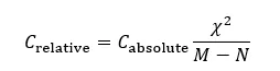
when the residual-degree-of-freedom denominator is available.

If the data owner cannot say which meaning was intended, the appropriate maintenance outcome is not to pick whichever flag gives more comfortable error bars. The uncertainty label should be held for review until the meaning and provenance of sigma are established. For a broader treatment of statistical uncertainty and regression assumptions, Refonte’s statistics article discusses the surrounding statistical judgment; the present question is narrower and specific to SciPy’s covariance normalization.

Distinguish sigma from the weights in the objective

For one-dimensional sigma, SciPy’s API says the entries are standard deviations of errors in ydata, and the minimized quantity is the sum of squared residuals divided by sigma**2. That means the corresponding influence is proportional to

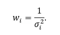
So “relative weights” and “relative sigma values” move inversely: doubling one observation’s sigma reduces its inverse-variance weight to one quarter.

That distinction matters operationally. A vector of raw variances is not interchangeable with a vector of standard deviations, and a vector of precision weights is not a drop-in replacement for sigma unless it is converted explicitly. The authored fixture below assumes synthetic sigma values with this documented standard-deviation interpretation. It does not demonstrate that those values came from a trustworthy measurement process.

Trace the covariance policy through the documented API

The omitted absolute_sigma argument and explicit absolute_sigma=False are the same documented API mode. In SciPy 1.17.0, the function signature sets absolute_sigma=False; the manual says only the relative magnitudes of sigma matter in that mode. By contrast, absolute_sigma=True makes pcov reflect the absolute supplied scale.

The parameter fit and the covariance normalization should be treated as separate stages conceptually. A one-dimensional sigma changes the least-squares criterion because the residuals are divided by sigma. The analytic Jacobian supplied by the caller is also scaled internally according to sigma; the SciPy manual explicitly says a callable Jacobian “will be scaled according to provided sigma.” In this fixture, the user function returns the unscaled derivatives [x, 1]; the library applies the response-error scaling.

The tagged SciPy 1.17.0 implementation makes that pathway concrete. For a scalar or one-dimensional sigma, minpackpy.py sets transform = 1.0 / sigma, wraps the residual function and wraps the Jacobian with that transform, then routes method='lm' through leastsq.

After the LM call, the wrapper computes the squared cost from infodict['fvec']. If absolute_sigma is false and the number of residual values exceeds the number of fitted parameters, it multiplies pcov by cost / (ysize - p0.size). If the denominator would have zero residual degrees of freedom, the implementation instead fills pcov with infinity and emits OptimizeWarning.

Here, M is the number of observations and N is the number of fitted parameters. Most cases use M=5, N=2, so M-N=3. The two-point boundary cases use M=N=2.

Keep low-level curvature and returned covariance separate

SciPy’s leastsq documentation describes its cov_x as a curvature-related inverse-Hessian approximation and says that, to obtain a parameter covariance, it must be multiplied by the variance of the residuals; it directs readers back to curve_fit.

That description belongs to the lower-level interface. The curve_fit wrapper performs its own covariance handling and, in relative mode, applies the residual factor before returning pcov. Multiplying an already returned relative-mode pcov by residual variance a second time would therefore change the result and would not reproduce the documented wrapper contract.

This is also why a source review should distinguish implementation layers. leastsq explains where the LM curvature estimate comes from; curve_fit defines what the caller ultimately receives under absolute_sigma. In the bounded fixture below, no private SciPy function is called directly.

Pin the runtime and construct an independent expectation

The supplied reference run was prepared on 2026-11-04 with Python 3.12.14, NumPy 2.3.5 and SciPy 1.17.0 on Linux 6.18.57 x86_64/glibc 2.39. The source file was reported as 144 lines and 686 whitespace-separated words with SHA-256:

b641978dec1c79910ffe03deae4f420c645270f05640fc2a44fcd667d374940d

The run started at 08:23:35.133557 UTC, finished at 08:23:35.178100 UTC, exited with status 0 and reported PASS_10_CASES. Those timestamps are provenance, not performance measurements, and the checksum identifies source bytes rather than proving that a particular process executed them.

For a standalone reproduction, save the source below as ml_curve_fixture.py. A matching package setup can be created with:

python3.12 -m venv .venv-curve
.venv-curve/bin/python -m pip install numpy==2.3.5 scipy==1.17.0
.venv-curve/bin/python ml_curve_fixture.py > ml_curve_results.json 2> ml_curve_stderr.txt

A command named python3.12 does not by itself guarantee patch version 3.12.14, so record the interpreter version from the generated JSON. NumPy and SciPy pins also do not constitute a complete binary or transitive dependency lock. Keep the process status, stdout JSON and stderr together with the source. For broader background on the ecosystem, Refonte’s overview of Python libraries for scientific computing discusses NumPy and SciPy’s roles at a higher level.

The supplied observations below remain the reference observations. No different interpreter or platform should be silently substituted and described as though it were that run.

Derive the two-parameter oracle without calling the optimizer

The oracle computes weighted straight-line normal equations using fractions.Fraction. It consumes only the authored literal x, y and sigma values. It does not consume fitted parameters, SciPy residuals or SciPy covariance.

For weights , it forms the weighted sums

solves the two-by-two normal equations for slope and intercept, and inverts the same two-by-two information matrix analytically. That provides an independent expected parameter vector and base covariance for every case.

This is consistent with the standard analytical straight-line least-squares construction described by NIST, which derives slope and intercept from the normal equations. NIST also gives the residual-scale denominator n - p , corresponding here to M - N , when estimating a residual standard deviation.

For the five-point noisy unit-sigma case, the exact oracle gives slope 2, intercept 1, weighted residual sum of squares 14, and residual degrees of freedom 3. The check is deliberately small and exact; it is not a general-purpose regression validator.

Run the complete covariance-scaling laboratory

The following is the complete supplied source. It performs ten outer curve_fit calls, compares each fit with the independent Fraction oracle, verifies selected cross-case relationships, checks the three input arrays for mutation and records warnings, solver status, covariance finiteness and environment metadata.

"""Owned covariance-scaling controls; no calibrated-uncertainty approval."""
import hashlib, json, platform, sys, warnings
from datetime import datetime, timezone
from fractions import Fraction as F
from pathlib import Path
import numpy as np
import scipy
from scipy.optimize import OptimizeWarning, curve_fit

X = (-2, -1, 0, 1, 2)
NOISY_Y = (-2, -3, 3, 1, 6)
EXACT_Y = (-3, -1, 1, 3, 5)
ONE = (1, 1, 1, 1, 1)
TEN = (10, 10, 10, 10, 10)
CASES = [
    ('F01', X, NOISY_Y, ONE, None),
    ('F02', X, NOISY_Y, ONE, False),
    ('F03', X, NOISY_Y, TEN, False),
    ('F04', X, NOISY_Y, ONE, True),
    ('F05', X, NOISY_Y, TEN, True),
    ('F06', X, NOISY_Y, (1, 1, 2, 1, 1), True),
    ('F07', X, EXACT_Y, ONE, False),
    ('F08', X, EXACT_Y, ONE, True),
    ('F09', (-1, 1), (-1, 3), (1, 1), False),
    ('F10', (-1, 1), (-1, 3), (1, 1), True),
]

def require(ok, label):
    if not ok:
        raise RuntimeError(label)

def close(actual, expected, label):
    a, e = np.asarray(actual, dtype=float), np.asarray(expected, dtype=float)
    require(a.shape == e.shape and np.allclose(a, e, rtol=1e-10, atol=1e-12), label)

def line(x, slope, intercept):
    return slope*x + intercept

def jacobian(x, slope, intercept):
    return np.column_stack((x, np.ones_like(x)))

def oracle(xs, ys, sigmas, absolute):
    x, y = list(map(F, xs)), list(map(F, ys))
    w = [1/F(s)**2 for s in sigmas]
    sw = sum(w)
    sx = sum(q*t for q, t in zip(w, x))
    sy = sum(q*t for q, t in zip(w, y))
    sxx = sum(q*t*t for q, t in zip(w, x))
    sxy = sum(q*t*u for q, t, u in zip(w, x, y))
    det = sw*sxx-sx*sx
    require(det > 0, 'Authored straight-line design must have full rank')
    slope, intercept = (sw*sxy-sx*sy)/det, (sxx*sy-sx*sxy)/det
    base = [[sw/det, -sx/det], [-sx/det, sxx/det]]
    chi = sum(q*(u-slope*t-intercept)**2 for q, t, u in zip(w, x, y))
    dof = len(x)-2
    if not absolute and dof == 0:
        covariance = [[float('inf')]*2 for in range(2)]
    else:
        factor = F(1) if absolute else chi/dof
        covariance = [[float(v*factor) for v in row] for row in base]
    return [float(slope), float(intercept)], covariance, float(chi), dof

def matrixjson(matrix):
    return [[float(v) if np.isfinite(v) else '+inf' for v in row] for row in matrix]

def main(report):
    require(np.__version__ == '2.3.5' and scipy.__version__ == '1.17.0',
            'Recorded NumPy/SciPy package baseline required')
    numerical = {}
    for identity, xs, ys, sigmas, mode in CASES:
        expected_p, expected_c, expected_chi, dof = oracle(xs, ys, sigmas, bool(mode))
        x, y, sigma = [np.asarray(v, dtype=np.float64) for v in (xs, ys, sigmas)]
        snapshots = [v.copy() for v in (x, y, sigma)]
        options = {} if mode is None else {'absolute_sigma': mode}
        with warnings.catch_warnings(record=True) as caught:
            warnings.simplefilter('always')
            report['curve_fit_calls'] += 1
            popt, pcov, info, message, ier = curve_fit(
                line, x, y, p0=[0., 0.], sigma=sigma, method='lm',
                jac=jacobian, full_output=True, options)
        close(popt, expected_p, identity+' parameter oracle')
        close(pcov, expected_c, identity+' covariance oracle')
        chi = float(np.sum(info['fvec']2))
        close(chi, expected_chi, identity+' residual criterion oracle')
        require(ier in (1, 2, 3, 4), identity+' solver status')
        require(all(np.array_equal(a, b) for a, b in zip((x, y, sigma), snapshots)),
                identity+' input arrays changed')
        warning_records = [{'category': type(w.message).__name__, 'message': str(w.message)}
                           for w in caught]
        if identity == 'F09':
            require(bool(caught) and all(isinstance(w.message, OptimizeWarning) for w in caught),
                    identity+' missing covariance warning')
        else:
            require(not caught, identity+' unexpected warning')
        numerical[identity] = (popt.copy(), pcov.copy())
        report['cases'].append({
            'case': identity, 'x': list(xs), 'y': list(ys), 'sigma': list(sigmas),
            'absolute_sigma_argument': 'omitted' if mode is None else mode,
            'expected_parameters': expected_p, 'observed_parameters': popt.tolist(),
            'expected_covariance': matrix_json(expected_c),
            'observed_covariance': matrix_json(pcov),
            'expected_chi_squared': expected_chi, 'observed_chi_squared': chi,
            'residual_degrees_of_freedom': dof, 'solver_status': int(ier),
            'solver_message': message, 'warnings': warning_records,
            'finite_covariance': bool(np.isfinite(pcov).all()),
            'inputs_preserved': True, 'status': 'MATCHED_NUMERICAL_CONTRACT',
        })

    close(numerical['F01'][1], numerical['F02'][1], 'Default matches explicit False')
    close(numerical['F03'][1], numerical['F02'][1], 'Relative scale invariance')
    close(numerical['F05'][0], numerical['F04'][0], 'Uniform sigma scaling parameters')
    close(numerical['F05'][1], 100*numerical['F04'][1], 'Absolute covariance scale')
    close(np.sqrt(np.diag(numerical['F05'][1])),
          10*np.sqrt(np.diag(numerical['F04'][1])), 'Parameter error scale')
    close(numerical['F02'][1], numerical['F04'][1]*float(F(14, 3)), 'Residual rescaling')
    close(numerical['F03'][1], numerical['F05'][1]*float(F(14, 300)),
          'Residual rescaling after sigma times ten')
    close(numerical['F06'][0], [2, float(F(11, 17))], 'Nonuniform-weight positive control')
    require(not np.allclose(numerical['F06'][0], numerical['F04'][0]),
            'Nonuniform weights did not change this fit')
    require(report['curve_fit_calls'] == 10
            and [r['case'] for r in report['cases']] == [f'F{i:02}' for i in range(1, 11)],
            'Case inventory')
    report.update(status='PASS_10_CASES', reconciliation={
        'default_equals_false': True, 'relative_sigma_times_ten_covariance_unchanged': True,
        'absolute_sigma_times_ten_covariance_factor': 100,
        'absolute_sigma_times_ten_parameter_error_factor': 10,
        'nonuniform_sigma_changes_this_fitted_intercept': True,
        'residual_rescaling_checked_at_both_uniform_scales': True,
    })

if name == '__main__':
    report = {'status': 'HOLD', 'cases': [], 'curve_fit_calls': 0,
              'started_utc': datetime.now(timezone.utc).isoformat(),
              'source_sha256': hashlib.sha256(Path(__file__).read_bytes()).hexdigest(),
              'environment': {'python': sys.version, 'platform': platform.platform(),
                              'numpy': np.__version__, 'scipy': scipy.__version__}}
    try:
        main(report)
    except Exception as error:
        report['error'] = {'type': type(error).__name__, 'message': str(error)}
    report['finished_utc'] = datetime.now(timezone.utc).isoformat()
    print(json.dumps(report, indent=2, allow_nan=False))
    sys.exit(0 if report['status'] == 'PASS_10_CASES' else 1)

The fixture’s comparison tolerance (rtol=1e-10, atol=1e-12) is appropriate only as a declared acceptance rule for this small example. It is not a universal numerical-analysis standard. Likewise, ten calls means ten outer invocations of curve_fit, not ten evaluations of the model or Jacobian.

The script checks the three caller arrays x, y and sigma for preservation. It does not claim that no other process state can change. It serializes nonfinite covariance entries as the string "+inf" only after comparison because JSON has no portable finite-number representation for positive infinity under allow_nan=False.

The experiment also deliberately treats incomplete evidence as failure. If an import, source-file read or earlier operation fails before useful JSON can be written, absence of a complete report is not evidence of success. An unexpected result should be investigated rather than forcing the oracle to agree.

Reconcile all ten cases before assigning an interpretation

The supplied reference matrix is:

The analytical matrices have zero off-diagonal entries in these symmetric designs. Observed floating-point matrices may contain tiny off-diagonal residues rather than exact symbolic zeros, so the fixture compares within declared tolerances rather than requiring bitwise equality.

Every row matched its independent per-case Fraction expectation in the supplied run. PASS_10_CASES also confirms the cross-case invariants: omitted mode equals explicit false, uniform tenfold sigma scaling leaves relative-mode covariance unchanged, absolute-mode covariance scales by 100, absolute-mode parameter-error magnitudes scale by ten, and the selected nonuniform sigma change modifies this fitted intercept.

Crucially, the aggregate status includes F09’s deliberately nonfinite covariance. PASS_10_CASES therefore means “the numerical behavior matched the expected contract,” not “ten uncertainty estimates are fit to publish.” That separation is the central review discipline for the rest of the article.

Keep fitted coefficients separate from the covariance convention

Cases F01 through F05 all fit the same line: slope approximately 2, intercept approximately 1, within the declared numerical tolerances. Yet they do not all return the same covariance.

That is expected. With uniform sigma, multiplying every value by the same positive constant multiplies the entire weighted least-squares objective by a positive constant. For this fixed full-rank linear problem, multiplying an objective by a common positive constant does not move its exact minimizer. The fitted coefficients therefore remain the same analytically.

That argument is about this objective and design; it should not be promoted into a claim that every floating-point nonlinear solver will traverse identical iterates or return bit-for-bit identical coefficients under every common rescaling. SciPy itself describes curve_fit as nonlinear least squares and describes pcov as an approximate parameter covariance based on a local linearization around the optimum.

The distinction also separates this question from the earlier Refonte workflow on keeping a declared regression design consistent. That article concerns prediction-time design construction and constant-column detection. Here the design never changes: there is always a slope coordinate and an intercept coordinate, the Jacobian retains full column rank, and no prediction batch is being regrouped.

So an unchanged fitted line is weak evidence for the covariance contract. A reviewer who sees [2, 1] in F02, F03, F04 and F05 still cannot infer whether the report preserved supplied absolute response-error scale or used residual-normalized relative sigma.

Explain the uniform-sigma cancellation with the authored numbers

The cancellation is easiest to see before considering any general matrix formula.

For

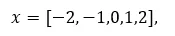
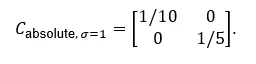
the model Jacobian has columns x and 1. With unit sigma, the information matrix is

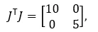
so its inverse in slope/intercept order is

For the noisy response

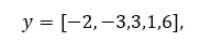
the fitted line is 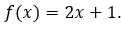. The authored residuals using the article’s y-f convention are

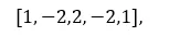
whose squared sum is 1 + 4 +4 +4 + 1 = 14

With five observations and two fitted parameters, M - N = 3. Therefore relative mode gives

SciPy’s full-output fvec uses the opposite sign for one-dimensional sigma: (f(x,*popt)-ydata)/sigma. The documentation states that sign convention explicitly. Squaring removes the sign, so the criterion remains 14.

Apply the rescaling equation only with positive residual degrees of freedom

Now multiply every sigma by ten.

Under absolute_sigma=True, every Jacobian row is divided by ten, so the information matrix is divided by 100 and its inverse is multiplied by 100:

Meanwhile the weighted squared residual criterion is divided by 100:

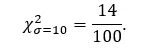
Relative mode therefore gives

The factor of 100 in absolute covariance cancels the factor of 1/100 in the residual criterion:

That is the F02/F03 invariance. It is exactly the behavior described by the SciPy formula for absolute_sigma=False when M > N .

Under absolute_sigma=True, there is no residual-scale cancellation. F05 is 100 times F04 in covariance, and therefore sqrt(diag(pcov)) is ten times larger. Only sigma changed here. No conversion of the physical units of x or y was performed.

Change relative weights as a positive control

Uniform rescaling could be misread as evidence that SciPy ignored sigma. F06 prevents that interpretation.

The only change from the baseline noisy case is the center observation’s sigma:

Because weights are inverse-square in sigma, the center observation’s weight changes from 1 to 1/4; the other four weights remain 1. This is a change in relative weighting, not merely a common scale factor.

The exact Fraction oracle gives slope 2 and intercept

The slope remains 2 because of the particular symmetric x layout and the authored values. The intercept does move, and the script explicitly checks that the F06 parameter vector differs from F04. That is a positive control showing that one-dimensional sigma participates in the fit.

The absolute-mode covariance is

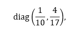
and the weighted residual criterion is

The result reconciles independently because the oracle computes the weighted sums directly from the authored literals.

NIST’s weighted-least-squares discussion makes the same high-level distinction: weights determine observations’ relative influence, and different sets of absolute weights can have identical effects when their relative pattern is unchanged. It also warns that the appropriateness and accuracy of estimated weights are a separate issue.

F06 therefore establishes only a narrow point: this particular nonuniform change moves this fitted intercept. It does not establish that every change in weighting must move every parameter, and it certainly does not establish that the authored weight pattern is physically correct or statistically superior.

Interpret zero residual covariance without claiming certainty

F07 and F08 use exact-line responses:

For the fixed design, these points lie exactly on

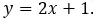
Both modes therefore return parameters [2,1], and the residual criterion is numerically zero in the supplied reference run.

With absolute_sigma=False, the covariance starts from the curvature matrix and is multiplied by the residual scale. Because the residual criterion is zero and M - N = 3, the scale factor is zero. F07 therefore returns a numerical zero covariance matrix.

With absolute_sigma=True, residual magnitude does not replace the supplied response-error scale. F08 retains

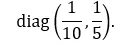
Neither matrix licenses a claim of perfect physical knowledge.

The F07 zero matrix is a direct numerical consequence of combining an exact synthetic line with residual-based covariance normalization. The observations are deterministic literals; there is no repeated-sampling experiment, measurement distribution, instrument calibration or uncertainty-validation study behind them.

Conversely, the nonzero F08 matrix does not prove that sigma=1 is a trustworthy measurement standard deviation. absolute_sigma=True means “use the scale supplied under this contract,” not “verify that the supplied scale is correct.” SciPy calls the result an estimated approximate covariance and notes that its interpretation relies on a local linear approximation for nonlinear models.

A reviewer should therefore preserve what was observed and the assumptions that generated it rather than choosing the matrix that looks more reassuring. Zero covariance in this fixture is not a scientific-certainty certificate, and finite covariance under True is not a calibration certificate.

Separate residual degrees of freedom from parameter identifiability

F09 and F10 are the most important boundary cases in the ledger.

They use two distinct predictor values: x = [-1,1] and exact responses y = [-1,3]

With two parameters (slope and intercept), those two distinct points identify the unique line y = 2x + 1

The two-column design is full rank. There is no algebraic ambiguity about the parameter vector.

But there are also exactly two observations and two fitted parameters:

M - N = 2 - 2 = 0

That means there are no residual degrees of freedom from which the relative-mode wrapper can estimate a residual scale through cost/(M-N).

In SciPy 1.17.0’s tagged implementation, the relative-mode branch checks whether ysize > p0.size. If not, it fills pcov with infinity and marks covariance estimation for an OptimizeWarning. The supplied reference observation for F09 is therefore an all-positive-infinity covariance plus one OptimizeWarning.

With absolute_sigma=True, the residual denominator is not needed. The supplied unit sigma scale is retained, and the exact inverse information matrix is

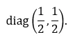
That is F10.

Preserve the full-rank boundary case

Do not diagnose F09 as rank deficiency.

Rank deficiency and zero residual degrees of freedom are different conditions. Here the design identifies both coefficients, but the relative-scale convention has no leftover residual dimension from which to estimate the common scale. SciPy’s documentation separately notes that a non-full-rank LM Jacobian is another reason an infinity-filled covariance can occur; that is not the mechanism exercised by this fixture.

The maintenance questions should therefore stay separate:

1. Can the design identify the parameters?

2. Does residual normalization have positive residual degrees of freedom?

3. If an absolute scale is supplied, is that scale actually justified by measurement and model evidence?

F09 answers “yes, no, not assessed.” F10 answers “yes, not required for this normalization, not assessed.”

The fixture requires at least one OptimizeWarning for F09 and requires every captured warning there to be an OptimizeWarning. Every other case must produce no warnings. That is an expected laboratory outcome, not evidence that every warning in other regression problems should be treated the same way.

Distinguish covariance arithmetic from uncertainty qualification

The ten-case experiment establishes a precise numerical result: for this full-rank straight-line fixture, SciPy 1.17.0’s documented covariance normalization reconciles with an independent Fraction oracle, including uniform-scale cancellation under absolute_sigma=False, scale retention under True, one nonuniform-weight control, an exact-residual case and a zero-residual-degree-of-freedom boundary.

That is enough to validate a narrow API interpretation. It is not enough to qualify the uncertainty model behind a scientific report.

A domain review still has to ask where sigma came from, whether its units match the response, whether its relative pattern is defensible, whether observation errors are adequately represented by the assumed structure, whether the model form is suitable, and whether the observed data are representative of the use being claimed. NIST explicitly separates the mechanics of weighted least squares from the problem of knowing the weights accurately.

The same distinction appears in larger weighted-estimation contexts. Refonte’s article on weighted estimation in orbit-determination workflows discusses covariance, measurement weighting and model mismatch in a much broader application setting; none of those application-specific algorithms or heuristics are evidence for the SciPy fixture here.

Likewise, SciPy’s own manual describes pcov as approximate and warns that the parameter-error relationship can be inaccurate when the local linear approximation is poor. A successful LM status, a finite covariance matrix and exact reconciliation with this linear oracle therefore cannot establish calibrated coverage, nonlinear-model adequacy, predictive quality, or trustworthy real-world error scales.

This laboratory does not test correlated two-dimensional sigma, uncertainty in x, robust losses, bound-constrained fits or another solver. Those cases should not inherit conclusions from this one by analogy.

Decide whether to report, reject a label or hold for review

A reporting decision should start from the intended meaning of sigma, not from the magnitude of the returned matrix.

The first row requires a qualification: the residual-rescaling formula in this experiment applies only where . F09 demonstrates the boundary directly. SciPy 1.17.0 fills the covariance with infinity instead of applying a zero-denominator scale.

The second row also needs discipline. Selecting absolute_sigma=True does not validate the absolute standard deviations. It only tells the function to preserve their scale in the covariance calculation. The trustworthiness of that scale remains a domain question.

Keep numerical acceptance separate from permission to make a claim

PASS_10_CASES is an engineering acceptance state for this fixture. It says that the ten expected numerical contracts, warnings and cross-case relationships were observed in the supplied reference run.

It is not a business-approval or scientific-qualification function.

A nonzero process exit, partial JSON, missing case, unexpected warning or environment mismatch should trigger investigation. A reviewer should not delete F09 because infinity is inconvenient, rewrite the oracle to match an unexpected result, serialize infinity as though it were a finite JSON number, or multiply a relative-mode pcov by residual variance again to force a preferred convention.

The bounded reporting rule is simpler: first identify the intended sigma contract, then verify that the code path and returned covariance match that contract, then limit the published claim to the evidence actually reviewed.

Preserve the evidence when correcting an analytical report

When a covariance label is corrected, preserve enough evidence that a later reviewer can reconstruct why the interpretation changed.

A practical handoff record should retain:

• the original x, y and sigma values, together with their stated meanings and units;

• parameter order: here explicitly slope, then intercept;

• the model function and analytic Jacobian;

• whether absolute_sigma was omitted, False or True;

• Python, NumPy, SciPy and platform identification;

• the source checksum and exact source artifact;

• the complete case record, including warnings, solver status and covariance;

• the original report language and the corrected language.

That is consistent with the broader discipline of preserving reproducible evidence in data-science projects, although the present workflow is intentionally narrower than the project lifecycle described there.

Ownership should also be explicit. The measurement owner should establish what sigma represents and where it came from. The model owner should review the error and model assumptions that make a covariance interpretation meaningful. The implementation maintainer should verify the API arguments, environment and numerical reconciliation. The report reviewer should decide whether the wording is supported by that combined evidence.

For an existing mislabeled result, recover the intended contract before rerunning. If the report meant to preserve an externally justified absolute response-error scale but the call used the default, rerun with an explicit absolute_sigma=True only after that contract is confirmed. If the report meant relative scales with residual normalization, make that convention explicit instead.

A corrected report should be a new reviewed artifact. Preserve the prior result and its provenance rather than overwriting history, because the distinction between “the numbers changed” and “the interpretation changed” can matter in later review. This article does not claim that any deployment, rollback, historical-data repair or production migration was performed.

A switch from False to True should never be justified by a preference for larger or smaller standard errors. In the supplied experiment, scaling sigma by ten under True makes covariance 100 times larger by construction. That arithmetic says nothing about whether the larger matrix is more truthful.

Requalification is warranted when any input to the claim changes materially: the response data, model definition, sigma meaning, relevant SciPy behavior, solver settings or intended reporting use. A library upgrade should be identified rather than silently treated as equivalent to the reference environment, especially because this article’s source-level reasoning is tied to SciPy 1.17.0.

The oracle itself should not be promoted beyond its design. It verifies a two-parameter straight line with one-dimensional positive sigma and the specified covariance rules. Copying the script into a nonlinear or correlated-error workflow does not make it a general covariance validator.

The final handoff should therefore end with an auditable decision such as: “relative-scale covariance verified under SciPy 1.17.0; absolute measurement-scale interpretation not claimed,” or “absolute-scale mode verified numerically; sigma provenance remains with the measurement owner.” Any unresolved assumption should remain visible.

Continue with Python and statistical-modelling foundations

The opening question now has a bounded answer. In the supplied SciPy 1.17.0 experiment, multiplying every one-dimensional sigma value by ten leaves returned covariance unchanged when absolute_sigma is omitted or explicitly False, because the 100-fold increase in the curvature-based covariance is canceled by the 100-fold decrease in the weighted residual criterion. With absolute_sigma=True, that cancellation is intentionally absent: covariance scales by 100 and sqrt(diag(pcov)) scales by ten. This matches SciPy’s documented absolute_sigma contract and the tagged wrapper implementation.

The practical habit is not to memorize one preferred flag. State what the response-error scale is supposed to mean, make the mode explicit where reporting depends on it, retain the numerical evidence, and constrain the claim to what both the API check and domain review actually support.

For readers building the underlying Python and modelling skills, Refonte Learning’s Data Science & AI programme lists Python Data Science, Statistical Modelling, Model Optimization & Problem-Solving Techniques, EDA and Data Visualization, Machine Learning and Predictive Modelling, and application to industry projects among its competencies. The programme page also lists NumPy among tools discussed in its FAQ and describes a 3-month, 12–14-hours-per-week format, alongside training and internship certificates on successful completion. Those foundations can support further practice in analytical Python and numerical review; the programme page does not establish that this specific curve_fit laboratory or covariance-normalization workflow is taught.